I finished reading Build a Large Language Model (From Scratch) by Sebastian Raschka two months ago. It taught me a lot about the foundations of what happens inside a LLM but I was curious what Pytorch exactly does.

am I able to make my own?

I quite literally knew nothing and I quickly realized it is a lot more complex than I thought. So I decided to just start with having the bare minimum starting with CPU only (Pt 1).

plan

with the help of claude I clarified what I must do/learn for Pt 1

• tensors : basic operations and abilities
• autograd : compute graph and backpropagation
• modules: layers, losses, optimizers so I can train something
• transformer: attention, layernorm
• mess around and train some stuff.

I would also be doing this all in C++.

I also had some basic tests for each step. In hindsight, I would have been better starting with claude making more thorough tests cause a lot goes wrong near the end ...

tensors

stride and shape

I always understood tensors as multi-dimensional arrays but for some reason thought they were stored like multi-dimensional blocks in memory. Well in reality they are just stored as a 1D array in memory with almost a legend defining how to access the data within the multi-dimensional array. Mainly the shape and stride.

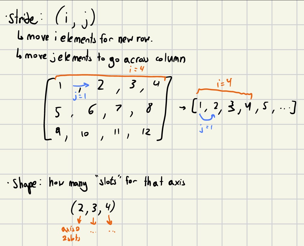
stride is the number of elements to skip in memory to get to the next element in a dimension. [i,j] -> i * stride[0] + j * stride[1] to get the index in the 1D array. Where the stride[0] is the number of elements to skip to get to the next row and stride[1] is the number of elements to skip to get to the next column.

shape is the number of elements in each dimension.

This approach allows for more flexibility where if we had to reshape the data doesn't directly change, rather the shape and stride are updated to reflect the new shape.

ops

Being new to C++ and overall no intuition it was all done very naively (will be improved in future parts!).

Add, subtract, and mul walk through index by index and apply the operation pretty straightforward.

Matmul was a bit more complex.

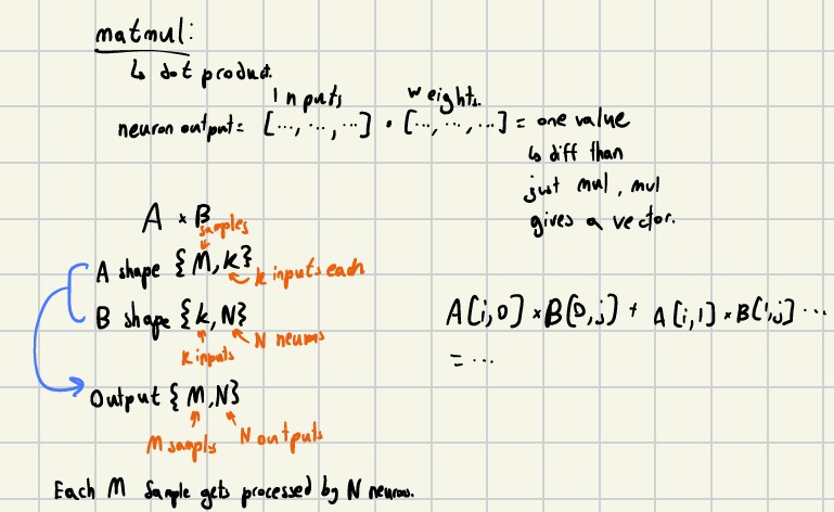
It was a triple-nested for loop computing dot product between rows and columns.

// simplified
for (int i = 0; i < M; i++) {
    for (int j = 0; j < N; j++) {
        float sum = 0.0f;
        for (int k = 0; k < K; k++) {
            sum += A[i][k] * B[k][j];
        }
        C[i][j] = sum;
    }
}

This a very brief summary of some basic operations for more check out in Tensor.cpp

It is important to note that none of this is fast. No SIMD, no cache blocking, and every op allocates for a new tensor. The goal was just to get something working and better understand before optimizing later on.

autograd

I always understood gradient was a way to measure how much a change in input affects the output (in the case of LLM, output = loss). But I never really understood how it was computed.

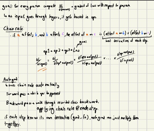
The core idea was that every tensor operation remembers how it was made so when we call backward() on the final tensor, using the chain rule, we compute the gradient of each tensor.

Every tensor holds a pointer to its inputs(inputs_) and a gradient function (grad_fn_) which knows how to use the upstream gradient to calculate the gradients for its input/operation. This makes the computation graph "imaginary" as it is just a series of tensors pointing at the tensors that created them, not an actual system storing the graph.

// simplified add operation example
output_tensor->inputs_ = {self, other}; // set the inputs of the operations so can track back
output_tensor->grad_fn_ = [self, other](const Tensor& upstream){
    if (self->requires_grad_) {
        self->init_grad();
        for (size_t i = 0; i < upstream.numel(); i++)
            //uses upstream gradient to compute gradient for the INPUTS 
            self->grad_->mutable_data()[i] += upstream.data()[i]; 

        // same for "other" tensor
    }
};

This was the add backward function since d(a+b)/da = 1, so the upstream gradient is just copied straight into the input's gradient. You might notice it's += because if the same tensor is used in operations in different places, the gradients accumulate together. The same is applied to the different ops but gradient calculation would be different.

In complete honesty, EVERY operation had to have a gradient calculation, that includes softmax, layernorm, and ... So I don't fully understand the math behind it all but understand the general concept and reasoning.

backpropagation

Reminder the whole goal of autograd is to compute the gradient of the loss with respect to all the parameters in the model (how much each weight affects loss). Once we have this we can update the weights accordingly to minimize loss (more later).

So the backward() does two things :

• build the process order (from loss backwards to the start)
• run each tensor's grad_fn_ (explained above) to compute gradients while passing down the upstream gradient.

// simplified
std::vector<Tensor*> order;
std::unordered_set<Tensor*> visited;

//Depth first search basically to collect the inputs we need to compute the gradient for in the right order.
std::function<void(Tensor*)> dfs = [&](Tensor* node){
    if (visited.count(node)) return;
    visited.insert(node);
    for (auto& input : node->inputs_)
        dfs(input.get());       
    order.push_back(node);
};

dfs(this);
std::reverse(order.begin(), order.end());  // DFS gives (start -> loss) we want (loss->start) so we reverse here !

// each node from steps before has their grad_fn called. and the upstream gradient is passed down.
// NOTE: their own gradient is stored in the tensor itself from the upstream call. 
for (auto& node : order)
    if (node->grad_fn_)
        node->grad_fn_(*node->grad_); 

This is where I got confused: How does passing its own gradient into its grad_fn_ compute the gradient for its inputs? The answer is the grad_fn_ is defined to use the upstream gradient to compute the gradient for its INPUTS. ex: initial upstream gradient is 1, so for add op the grad_fn_ will just copy the upstream gradient into its inputs. So by passing the upstream gradient down through each grad_fn_, every tensor ends up with the gradient it needs.

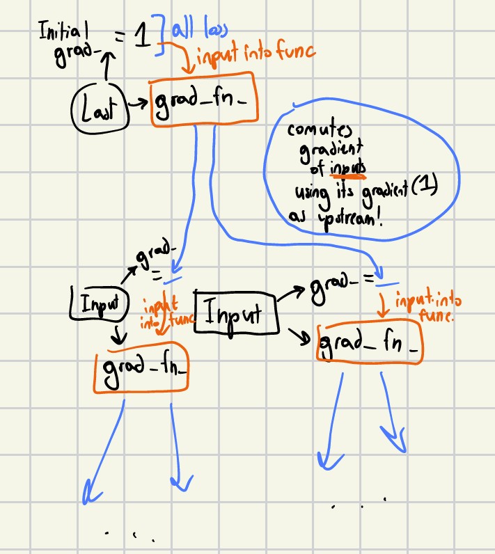
Similar to the tensor operations, performance is not good. Every grad_fn_ is a simple for loop and single-threaded. Common theme for part 1.

modules

Now with forward (tensor ops) and backward (autograd) working, we can start to build modules that can be used to actually TRAIN a model.

It's important to note the structure of each module:

• each has a forward() function that just runs the calculation
• also a parameters() function that returns all info used in that module.

linear, activation, sequential

Linear

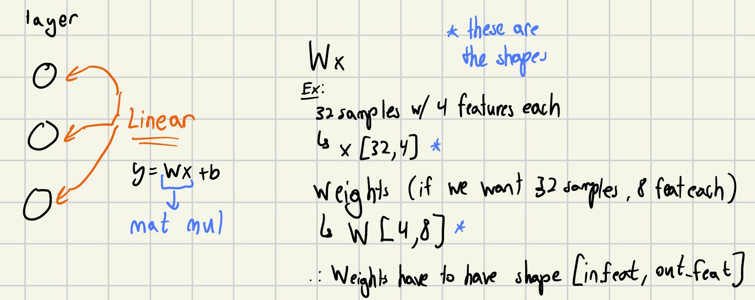
Linear is a simple linear transformation of the input.

where the weights W and bias b are learnable parameters. They are initialized randomly (didn't realize there is complexity to this and did come to bite me later on) and updated during training to minimize the loss. In the note above, it is good to note the shapes. Understanding the property of Matmul we know how to get he output shape given the input shape and the weight shape.

Activation Func

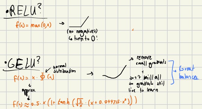
activation functions sit between layers (ex linear) and introduce non-linearity to the model. Think about if each layer is just linear transform and passed onto another linear transform, the whole model is just a linear transform. Leading to a model that cannot learn complex patterns. The two ones implemented are ReLU and GELU.

Relu is a simple function that outputs the input if it is positive and 0 otherwise. However, this isn't always the best choice as it can lead to "dead neurons (one output number)" where the gradient is 0 and the neuron never updates. We want as many neurons to be active so the model can learn. So there is GELU which is smooth and includes negative inputs (derivative is small but non-zero) so the neuron can still update.

The difference is graphed very roughly above.

NOTE: even this has its own grad_fn_ for autograd even though it is just a function and not a learnable param, it still needs to compute the gradient as the value changes and has to have the change reflected in later layers.

Sequential

It's just a container for the modules. It chains a list of layers together, forwarding each one's output to the next input.

There will be an example later on that puts everything together

loss and optimizer

The whole point of training a model is to minimize the loss. So we need a loss function to calculate how far off the model's prediction is and an optimizer to update the model's parameters to minimize the loss.

Loss

MSE is used for regression tasks where the target is a continuous number, not a category. So it measures how far each prediction is.

CrossEntropy, on the other hand, is used for classification. The model outputs a vector of probabilities for each class, and the target is the index of the correct class.

For example, if there's 90% probability on the correct class, log(0.9) is a small negative number → low loss. If there's only 1% probability on the correct class, log(0.01) is a large negative number → high loss.

Optimizer

Honestly I don't fully understand the math behind it but the idea is to use the gradient to update the parameters in a way that minimizes the loss. This is a good video explaining the different optimizers link

It holds a list of parameters from Sequential (above, a collection of layers and their parameters). After backward() is called, meaning all params have their gradients computed, step() from the optimizer reads the gradients and nudges each weight's value in a direction that reduces loss.

spiral

Here is a good example of putting everything together and hopefully making more sense. The task is to predict what class a point belongs to given in a spiral shape. This is challenging because a spiral is not linearly separable since they intertwine.

//SIMPLIFIED EXAMPLE
//assume we have a input tensor shape (N, 2) where N is the number of points and 2 is the x,y coordinates.
//assume we also have a target tensor shape (N,) where N is the number of points and each value is the class index (0,1,2) for each point.

//initalize model 
auto model = std::make_shared<Sequential>(std::vector<std::shared_ptr<Layer>>{
    std::make_shared<Linear>(2, 16),// y = xW + b , where input feat = 2, output feat = 16
    std::make_shared<GELU>(), //activation function to introduce non-linearity
    std::make_shared<Linear>(16, 16),
    std::make_shared<GELU>(),
    std::make_shared<Linear>(16, num_classes) //in this case 3 classes with logits (raw) output (we could use softmax to turn into probabilities which is what CrossEntropy does)
});

CrossEntropy loss_fn;
AdamW optimizer(model->parameters(), 0.01f);

//training loop (1000 loops/epochs)
for (int epoch = 0; epoch < 1000; ++epoch){
    auto logits = model->forward(input_tensor); //1. make prediction passing through the sequential model (ABOVE)
    auto loss = loss_fn.forward(logits, target_tensor); //2. compute loss between prediction and target

    loss->backward(); //3. backpropagation to compute gradients for all parameters in the model
    optimizer.step(); //4. optimizer updates the parameters using the computed gradients to minimize the loss
    optimizer.zero_grad(); //5. reset gradient to zero for the next epoch
}

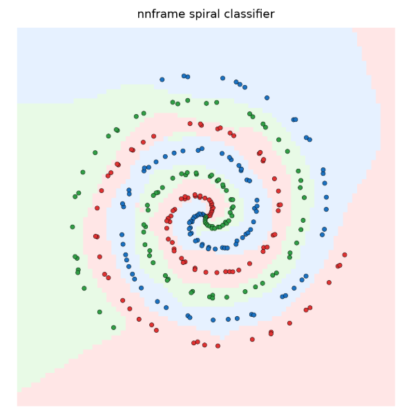
The result gave us a nice spiral shape where each point was classified correctly and you can see the pattern between colours. The dots are the input with their target data we gave. Our model learned the complex pattern.

transformer

Well it is proven you could build a general neural network but to make a LLM we would need to implement a transformer.

It's different as it is designed to take in a sequence of tokens (characters, words, subwords, etc) and predict what the next token should be. The overall goal is still a work in progress likely for a future part (need faster and optimized compute likely GPU🤯) but some main blocks was completed.

First an embedding layer:

Sentence -> cutup into tokens (words, subword, ex: " i have a dog" -> ["i", "have", "a", "dog"]) -> each token is mapped to a vector of numbers (embedding) -> the sequence of embeddings is passed into the transformer.

This is probably the best reasource to explain transformer and attention link. But here is my attempt to explain it in my own words.

attention

The main challenge attention solves is that in a sequence, not all tokens are equally important. Naturally in a paragraph words next to certain words have changed meanings and we need the embeddings to reflect that.

Essentially attention is comparing each token to every other token in the sequence and computing a weight for each token based on how important it is to the current token.

Each token is transformed into three vectors: Query, Key, and Value.

Query

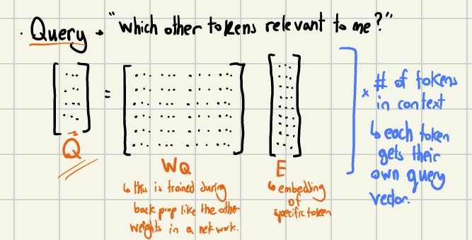
The query vector is almost like a question for the current token, where the other tokens are the answers. Reminder that Wq is a learnable parameter that is updated during training.

Key

The key vector represents the information (answer to query) for the current token. Wk is also a learnable parameter that is updated during training.

How does Query and Key exactly connect?

We established there is a relationship. Here is how they impact the attention score.

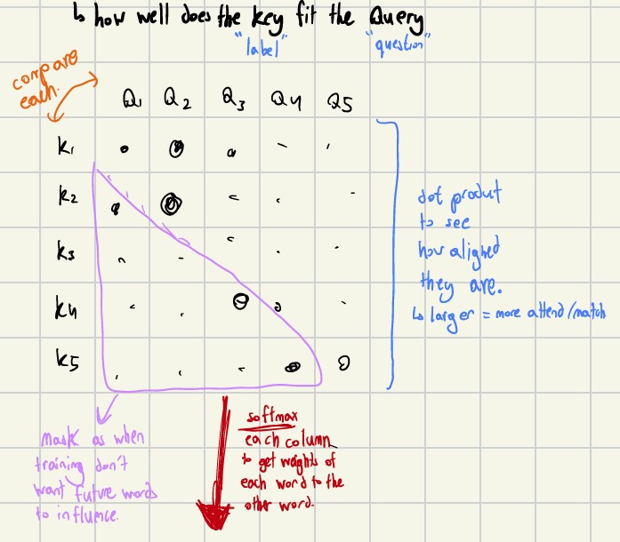
Every token's Query is compared to every other token's Key using dot product. This answers the question "how close does the Key answer the Query" because imagine 2 vectors, if they are pointing in the same direction the dot product is large meaning the Key is a good answer to the Query. If they are pointing in opposite directions the dot product is negative meaning the Key is a bad answer to the Query.

Future tokens are hidden so the model cannot cheat and look ahead ( -> current, not -> current -> future). Ex: "I have a cute fluffy cat and a mean dog" -> if we are predicting next token after "cute" the model should not be able to look ahead and cheat, it needs to learn the pattern of the sequence.

After the dot product is computed, softmax is applied to turn the scores into a probability distribution along each token. This is the attention weight for each token. The higher the weight, the more important that token is to the current token.

Value

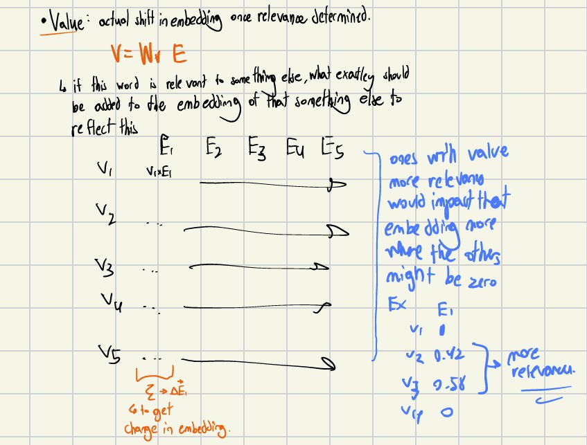
Value is the actual information of the token. Where Wv is also a learnable parameter that is updated during training.

The attention weights (from above, how Q connects to K) are used to scale the Value vector of each token, and the weighted sum of these scaled Value vectors is the output of the attention mechanism for the current token.

By taking the sum of the result for each token we get the change that needs to be applied to the current token's embedding to reflect the context of the sequence. Think of it shifting the vector towards a better representation of itself.

It really comes down to this formula.

Note: Wq, Wk and Wv are learnable as they are tensor operations and have gradients computed during backpropagation. During the optimizer step, they are updated to minimize the loss. Nothing new but each iteration changes weight in turn changes the embeddings to match the context of the sequence better.

layernorm

Following this link formula for layer norm.

I also don't fully understand the math behind it but the idea is to normalize the input to a layer so that it has a mean of 0 and a standard deviation of 1. This helps with training stability since the values don't get to large/small as they pass through the layers. It also has two learned params gamma and beta which are used to scale and shift the normalized values.

positional encoding

Same for positional encoding (😭) link

Attention itself doesn't have a sense of order like it compares every token to every token (dot product), so even if we lets say shuffle the input sequence it wouldn't actually change the attention score. This is different than masking. Masking is just hiding future tokens so the model cannot cheat while positional encoding is giving the model context on the order of the sequence.

Positional encoding adds a pattern to each token before it enters the transformer. Using the embedding's index and dimension, it either uses sin (even index) or cos (odd index) to change the value of the embedding. This pattern is unique for each position and dimension so the model can learn to recognize the order of the sequence.

transformer block

With all the pieces made we need to wire them together.

// simplified
//assumes we have embeddings and positional encoding added as the input. 

TensorPtr pre_norm_input = layer_norm1_.forward(input);
TensorPtr attn_output = self_attention_.forward(pre_norm_input); 
TensorPtr residual1 = attn_output->add(input); //output of attention is change in embedding so we add it to the original        

TensorPtr pre_norm2 = layer_norm2_.forward(residual1);
TensorPtr linear_output1 = linear1_.forward(pre_norm2);
TensorPtr gelu_output = GELU().forward(linear_output1);
TensorPtr linear_output2 = linear2_.forward(gelu_output);
TensorPtr output = linear_output2->add(residual1); //update embeddings again.       

They both follow the pattern of layer norm -> attention/linear -> residual connection.

We understand why attention is needed but why linear?

Referencing above in previous sections, the linear layers are essentially there to almost give each token a "voice" to express itself. Where as the attention is comparing between tokens, the linear layer is just transforming the token itself as the model trains.

By stacking a handful of these transformer blocks together each updating the embeddings, we can use the final embedding to actually predict the next token.

next steps

The transformer stuff is still a work in progress and the end goal is to train a small LLM. But as I mentioned throughout, the performance is not good and I need to optimize.

I guess the real motivation to start this was wanting to learn things like inference, CUDA, and MLsys. This project was more about understanding the foundations of what happens inside an LLM first. So next, I want to focus on the things I actually want to learn and implement.

Understanding my motivation, I often used claude to almost "skip" some gradient calculations and other stuff as I didn't feel like it was too important to understand the math behind those parts if not relevant.

But anyways, I am working on part 2.

Thanks !