Video Virality Predictor

June 2026

Over the past school year (Sept -> April) I was a part of Western AI and with a group of 5 we made a video virality predictor. It takes a youtube short and tries to predict the number of views.

Check out the report

View on GitHub

However I was very new to ML/AI so I decided to take a deep dive into what was implemented and share what I learned!

Embeddings

At the surface embedding is really just a way to turn complex into a numerical value, vector, so the mathematically you can determine how related based on how close they sit in that geometric space. All our embeddings were 768-dim vectors.

Text

Once the video's metadata (title,description, tags) and transcript were collected, we used a pretrained model called MiniLM. However is only produced a 384-dim vector, which we had 768-dim for the audio and video (later...).

So we concat the metadata embed with the transcript embed to get a 768-dim vector.

I remember my first instinct was doesn't this concat pollute the similarity measure? As in the score is now influenced by both halves equally, similar metadata but different transcript will have a high similarity score and visa versa. But after thinking about it, the creator's provided context describes what's happning with the video aswell meaning important context. It's an assumption that the metadata matches that of the content.

Audio

Using Wav2Vec2 we were able to extract a 768-dim vector from the audio.

It processes the audio by taking a sequence of tiny time slices (20ms) each producing its own 768-dim vector. To represent the entire audio with one vector, we take the mean of all the vectors.

Seems simple but there are many nuances.

By taking the mean, we are assuming that all parts of the audio are equally important. However, some parts of the audio may be more relevant to the video's content than others. For example, a loud FAAAHHHHH in the start of the video may be more important than a quiet background noise at the end.
The model was trained on 16 kHZ audio, but a typical video is 48 kHz. Meaning higher frequencies are lost giving a less accurate representation of the audio in the embedding.

Video

This was probably the most interesting embedding to me.

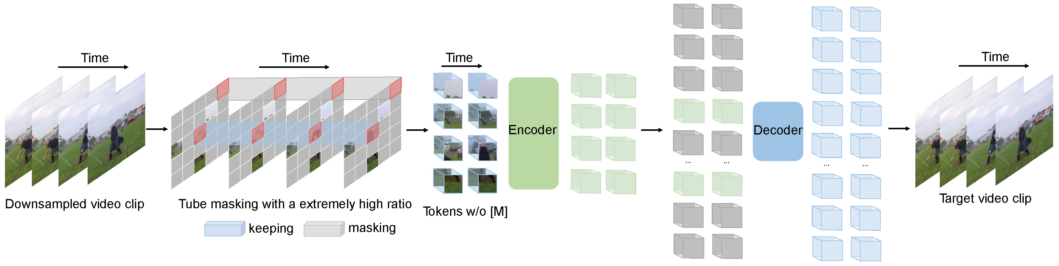
Using a sampling rate of 16, it would take 16 evenly spaced frames from the video and pass them through a pretrained model called VideoMAE.

#pick 16 evenly spaced frames from the full video
indices = np.linspace(0, len(frames) - 1, 16, dtype=int)
sampled = [frames[i] for i in indices]

The real weakness is typically some Shorts rely on rapid cuts/visual changes. 16 frames may miss those key moment. But at the same time, it is unrealistic to process all frames in a video, especially for longer videos. The model should still be able to capture the overall context of the video, such as static talking head, vs a fast-paced action scene.

After the frames are sampled, they are passed through the model to produce a 768-dim vector. Unlike audio, VideoMAE has a CLS token (summary vector) for the whole clip.

Multi-Modal Fusion

We need to combine the three embedding into a single vector to represent each video so the models can process.

Going with the simplest approach, we just concat the three embeddings with 2 additional masks, audio_present & video_present. This helped maintain all info from the three modalities, while also providing a way for the model to know if a modality is missing. video + audio is required, otherwise removed

\text{video}_{768} + \text{audio}_{768} + \text{text}_{768} + \text{audio\_present}_{1} + \text{video\_present}_{1} = \text{2306-dim vector}

Latent-Space Reduction

Why reduce at all -> Curse of Dimensionality

The larger the dimension, the slowly the data points become more sparse making it harder to find these relationships since the distance is so far apart becoming equally distant.

PCA (2306 -> 50)

A brief overview:

find the directions of max variance in the data and project everything onto those axis.
smaller signals that don't represent too much variance are dropped
linear transformation of the data to a new coordinate system

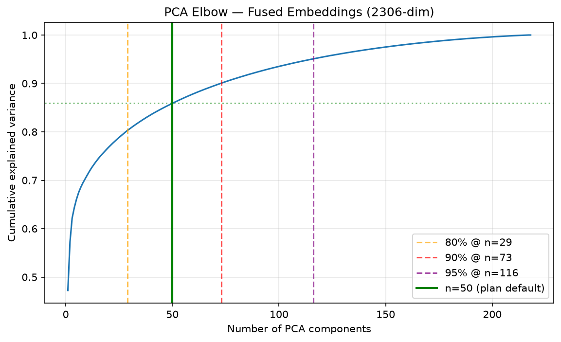
PCA elbow plot — Variance captured vs number of components

Above is a plot of the variance to number of components. Looking at the value of 50 around 86% of the variance was captured and after this point, the variance captured starts to plateau or components grew too large.

UMAP (50 -> 15)

Another brief overview: this still doesn't fully make sense

it makes a graph of nearest points (neighbors) and tries to find a low-dimensional representation of the data that preserves the local structure of the data.
non-linear transformation of the data to a new coordinate system

After removing the noise from PCA, we can now use UMAP to further reduce the dimension to 15.

X_umap15 = umap.UMAP(n_components=15, n_neighbors=50, min_dist=0.1).fit_transform(X_pca50)

Another question was: when you reduce the dimension so much how to make sure you not breaking relationships between points/videos?

neighbor overlap

By measuring the 15 nearest neighbors each video in the PCA-50 space and UMAP-15 space, we can measure how many of the neighbors are the same.

#fraction of neighbours preserved after reduction
overlap = neighborhood_overlap(X_pca50, X_umap15, k=15)

Clustering

Using K means, it picks K cluster centers at random and assigns every video to the nearest cluster center. Then move each center of cluster to the mean position of all videos assigned to it. It would repeat until the cluster center stops moving. Meaning the every video closer to thier own cluster center than any others.

Clustering should only be applied on PCA-50 because it is a linear transformation. So the distance between videos in the original 2306-dim is the same. However Umap-15 is not linear changes distance between points, so the clusters would not be accurate.

Well how to pick the K, number of clusters?

Inertia

Track the total distance of each video to its cluster center. With more clusters it would improve but at what point does it not have much improvement?

#lower = tighter clusters
for k in range(2, 16):
    km = KMeans(n_clusters=k)
    km.fit(X)
    print(f"K={k}: inertia={km.inertia_:.1f}")

Silhouette Score

Measure how close each video is to one another in the same cluster vs how far it is from videos in the nearest cluster

silhouettes[k] = silhouette_score(X, labels)
best_k = max(silhouettes, key=lambda k: silhouettes[k])

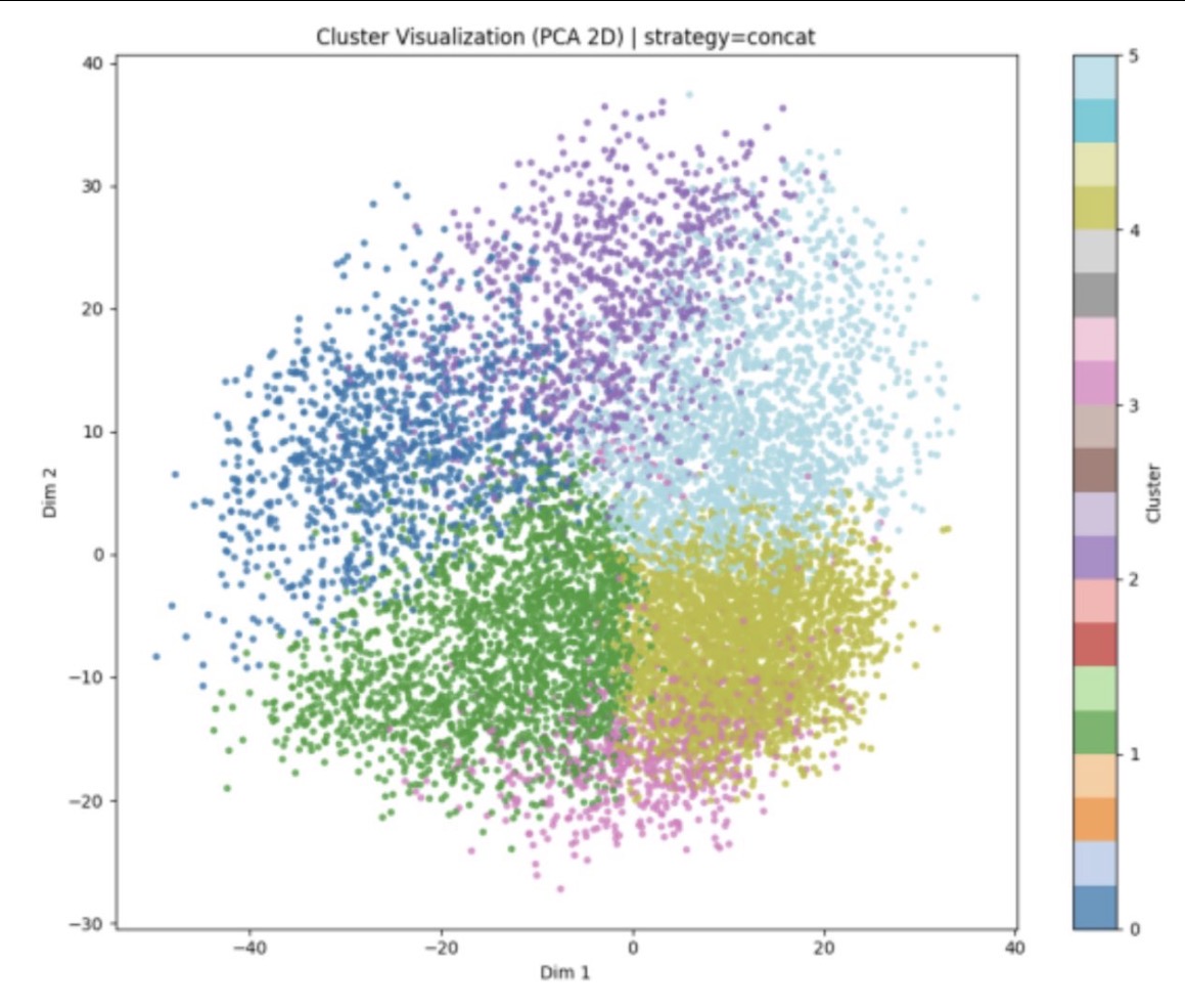
Cluster Interpretation

After clustering, the videos are grouped.

For each clustered video, we wanted to understand what human signals makes the video similar?

motion_mean
cut_rate_per_min
audio_rms_mean
audio_rms_std
visual_density

Although it wasn't the most detailed analysis, it gave us some signals of the video groups

Model Training

now to actually predicting the number of views some we used was Ridge Linear Regression, Gradient Boosted Decision Trees (GBDT), and Multi-Layer Perceptron (MLP).

but first we had to prevent data leakage. As some features in the metadata contains info that only exist after the video is published. For example, the number of likes, comments, and shares. So we removed those features from the training data. we don't want the model to build relationships that are cheating, more like == more views.

#only pull these specific columns from metadata -> everything else dropped
keep_meta = ["video_id", "target"] + [c for c in FEATURE_COLS if c in meta.columns]
meta = meta[keep_meta].copy()

Ridge Linear Regression

Linear models assume virality scales with each feature ex, channel_video_count more = more viral. This was treated as our baseline

Ridge minimises this loss:

\text{Loss} = \underbrace{\sum(y - \hat{y})^2}_{\text{how wrong}} + \alpha \cdot \underbrace{\sum \beta^2}_{\text{how big the weights are}}

The first part is the same as linear regressions, the error between predicted vs actual. the second part was the alphas...

Something I found challenging to get my head around was the application of RidgeCV and alphas.

#log-spaced so small and large values get equal attention
RidgeCV(alphas=[0.1, 0.3, 1, 3, 10, 30, 100])

Ridge is run multiple time with various alpha values. These alphas are the regularization strength. The higher the alpha, the more the model is penalized for having large weights. The lower the alpha, the less the model is penalized for having large weights. Basically it tries to find the best alpha that makes the model not rely too much on any one feature, making sure the weights are balanced.

Gradient Boosted Decision Trees

It builds a series of decision trees, where each tree tries to correct the mistakes of the previous tree by predicting the error. Using a learning rate of 0.05, the model slowly gets better cause with more trees it would be more generalized with smaller steps.

model = HistGradientBoostingRegressor(
    learning_rate=0.05,   # small correction per tree
    max_iter=500,         # 500 sequential trees
    max_depth=6,          # tree complexity limit
    min_samples_leaf=20,  # prevents overfit on small groups
    early_stopping=True,
)

Multi-Layer Perceptron

The concat MLP takes the full 2306-dim fused vector.

The architecture is :

nn.Sequential(
    nn.Linear(in_dim, 1024), nn.GELU(), nn.Dropout(0.2),
    nn.Linear(1024, 512),    nn.GELU(), nn.Dropout(0.2),
    nn.Linear(512, 256),     nn.GELU(), nn.Dropout(0.2),
    nn.Linear(256, 1),
)

Each layer halfs the number of neurons, with GELU because RELU perma kills neurons stopping them from learning. Dropout randomly zeros neurons for the forward pass making sure it doesn't rely on any single neuron.

The validation loss is monitored and stop when the model doesn't improve for 6 consecutive epochs. The model is then restored to the best state.

if val_loss < best_val_loss:
    best_state = model.state_dict() #save best weights
    no_improve = 0
else:
    no_improve += 1
    if no_improve >= patience: #6 epochs without improvement
        break

model.load_state_dict(best_state) #reload best, not final

What I Learned and Why

Quick:

Having clean data is more important than I thought.
It is super important to have structured data and a clear plan before starting. Constantly I was getting confused such as VideoIDs, URLS, or other names it quickly became messy.
Writing about something is a great way to force yourself to understanding better. Even though it may not be the best

I feel like something I realized as I continue to make more things that are difficult is that there is no right way to do things. That is why it is so important to ask questions so you can justify with yourself why you are doing something a certain way. Should we use this model? What about the loss function? How might the learning rate impact our model?

At the same time it doesn't mean you have to have every step figured knowing where you fell short is just as important to knowing why you made the choices you did.

As someone who overthinks a lot it was a good reminder...

I'll come back to clarify any section later as I gain more experience

References